 All Posts
Kedify Predictor: Explainable Forecasting with Jupyter Notebooks
September 02, 2026
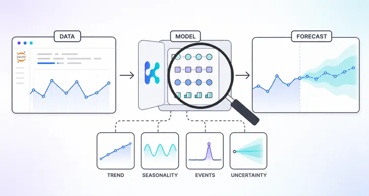
Make Predictive Autoscaling Forecasts Easier to Trust
Predictive autoscaling asks operators to let a forecast influence production capacity. That forecast should be inspectable, not something you accept on faith.
Kedify Predictor 0.1.6 can create an on-demand JupyterLab workspace for a MetricPredictor, connected to the metric history associated with that resource’s model. The included notebooks let you compare simpler forecasting baselines, evaluate behavior on held-out data, and test Prophet settings initialized from the current MetricPredictor configuration.
The comparison notebooks are diagnostic; MetricPredictor continues to use Prophet. Nothing you change in Jupyter updates the resource or publishes a trained model automatically. Applying configuration and requesting a retrain remain explicit steps.
This post walks through reproducing the workflow in a local k3d cluster, then compares the included forecasting techniques and shows how to test Prophet settings.
Make predictive autoscaling easier to trust.
Inspect metric history, compare forecasts, and test Prophet settings with Kedify Predictor.
Get Started1. Create a k3d Cluster
You need k3d, kubectl, and Helm. Create the local cluster:
k3d cluster create predictor-notebooksAdd the Kedify chart repository if it is not configured already:
helm repo add kedifykeda https://kedify.github.io/chartshelm repo update kedifykeda2. Prepare PostgreSQL
Notebook workspaces require Predictor to use PostgreSQL. The default SQLite configuration cannot safely provide the same metric store to independently scheduled notebook pods.
For this local example, create the database credentials and install PostgreSQL in the keda namespace:
kubectl create namespace kedakubectl create secret generic postgres-credentials -n keda \  --from-literal=postgres-password="$(xxd -l10 -ps /dev/urandom)" \  --from-literal=password="$(xxd -l10 -ps /dev/urandom)"# in prod use something like vault-secrets-operator / external-secrets / SOPS, etc. to manage secrets instead of a literal password
helm upgrade --install postgres \  oci://registry-1.docker.io/bitnamicharts/postgresql \  --version 18.8.12 \  --namespace keda \  --set auth.database=kedify \  --set auth.username=kedify \  --set auth.existingSecret=postgres-credentials \  --wait
Use a managed PostgreSQL instance and appropriately scoped credentials outside a disposable development cluster.
3. Install Kedify with Predictor Enabled
Predictor is a dependency of the Kedify Agent chart, so it can be enabled in the same values file instead of installed as a separate Kedify release. Obtain the organization ID and API key from the Kedify dashboard, then save the following as kedify-values.yaml:
clusterName: predictor-notebooks
agent:  orgId: '<YOUR_ORGANIZATION_ID>'  apiKey: '<YOUR_API_KEY>'
keda:  enabled: true  # enable raw-metrics gRPC API in KEDA  env:    - name: RAW_METRICS_GRPC_PROTOCOL      value: enabled    - name: RAW_METRICS_MODE      value: pollinginterval
kedify-predictor:  enabled: true  kedaPredictionController:    noSharedVolumes: true  db:    type: postgres    host: postgres-postgresql    name: kedify    user: kedify    existingSecret: postgres-credentials    existingSecretPasswordKey: password
Use Kedify Agent chart 0.6.9 or newer with kedify-predictor 0.1.6 or newer.
Install the umbrella chart:
helm upgrade --install kedify-agent kedifykeda/kedify-agent \ --namespace keda \ --values kedify-values.yaml \ --waitThis CSV-based example does not need a live KEDA metric subscription, but enabling KEDA leaves the cluster ready for a MetricPredictor whose source refers to a ScaledObject trigger.
4. Create a MetricPredictor
The following resource imports four weeks of samples at 30-second intervals. addTimestamps tells Predictor to generate timestamps because the CSV contains values without a time column.
kind: MetricPredictorapiVersion: keda.kedify.io/v1alpha1metadata: name: csv-source namespace: defaultspec: source: oneShotCsv: url: https://storage.googleapis.com/kedify-predictor/website_traffic_4weeks_30s.csv addTimestamps: true timestampPeriod: 30s timezone: Europe/Prague model: type: Prophet name: csv-source defaultHorizon: 10m retrainInterval: 1dSave it as metric-predictor.yaml, apply it, and wait for reconciliation:
kubectl apply -f metric-predictor.yamlkubectl wait --for=condition=Ready metricpredictor/csv-source --timeout=5mkubectl get metricpredictor csv-source -o wideFor this dataset, the CSV status should become IngestionOk. The import creates 80,640 samples, enough history for the daily and weekly patterns used throughout the notebooks.
5. Deploy the Notebook Workspace
Add the kedify.io/notebook=true annotation to the MetricPredictor:
kubectl annotate metricpredictor csv-source \ kedify.io/notebook=true --overwriteThe Predictor controller responds by creating a one-replica Deployment and a ClusterIP Service in the keda namespace. Their name combines the MetricPredictor name and namespace, so this example produces csv-source-default.
kubectl get deployment,service -n keda \  -l app.kubernetes.io/name=kedify-prophet-notebook
kubectl rollout status deployment/csv-source-default \  -n keda --timeout=2m
The resulting resources look like this:
NAME                                       READY   UP-TO-DATE   AVAILABLEdeployment.apps/csv-source-default        1/1     1            1
NAME                               TYPE        PORT(S)service/csv-source-default         ClusterIP   8888/TCP
If <metricpredictor-name>-<namespace> would exceed Kubernetes’ 63-character name limit, the controller truncates it and adds a hash. The label-based kubectl get command above finds the final name.
Each notebook pod receives the selected model name and PostgreSQL connection settings. It runs as a non-root user without a service account token. Its /workspace directory is backed by emptyDir, so download any changed notebooks or results that you want to keep.
6. Open JupyterLab
The Service is intentionally not exposed outside the cluster. Forward it to the loopback interface:
kubectl port-forward -n keda --address 127.0.0.1 \ service/csv-source-default 8888:8888Leave the command running and open http://localhost:8888. Start with 00-index.ipynb, then run a technique-specific notebook from top to bottom.
7. Compare the Included Forecasting Techniques
The workspace includes an index and nine executable notebooks:
| Notebook | Technique | What to look for |
|---|---|---|
01-simple-exponential-smoothing.ipynb | Simple exponential smoothing | Estimates a changing level with alpha. Multi-step forecasts are flat because it has no trend or seasonal state. |
02-double-exponential-smoothing.ipynb | Holt’s double exponential smoothing | Adds a local linear trend with alpha and beta. It works for non-seasonal trends but extrapolates a straight line. |
03-triple-exponential-smoothing.ipynb | Holt-Winters triple exponential smoothing | Adds a repeating seasonal component using alpha, beta, gamma, and a known period. It works best when the cycle remains stable. |
04-linear-regression.ipynb | Linear regression | Fits one global time-based slope. It is fast and interpretable but does not represent cycles or changing trends without more features. |
05-moving-averages.ipynb | Recursive moving average | Provides a useful short-horizon baseline. Longer recursive forecasts converge toward a constant as predictions replace observations in the window. |
06-arma-arima.ipynb | AR, MA, and ARIMA | Compares lagged values, lagged errors, and differencing. These methods can model stable short-term dependence but require selecting p, d, and q. |
07-dynamic-harmonic-regression.ipynb | Dynamic harmonic regression with ARIMA errors | Represents daily and weekly cycles with Fourier terms and models residual dependence with ARIMA. Seasonal periods and model orders must be chosen explicitly. |
08-fft.ipynb | FFT spectral forecasting | Finds dominant frequencies, filters components, aligns phase, and can extrapolate a trend. It is fast for stable periodic signals but has no changepoints, holiday effects, or calibrated uncertainty. |
09-prophet.ipynb | Prophet | Combines a flexible trend, changepoints, several seasonalities, holidays, custom events, and uncertainty intervals using Predictor’s production model-building logic. |
The simple models are useful because their limitations are visible. Linear regression reduces this traffic history to a single level and slope, missing the repeating intraday shape:
Holt-Winters adds level, trend, and one seasonal cycle. With an appropriate period it follows the repeating traffic, although the smoothing parameters still affect how quickly it reacts:
FFT approaches the same pattern in the frequency domain. The notebook makes phase alignment, frequency filtering, and trend handling explicit rather than treating the transform itself as a complete forecast:
Compare held-out scores and forecast shape together. A smooth fit over training data does not show how a method behaves on unseen samples, and the smallest error on one split is not necessarily the most stable choice for a production series.
8. Test Prophet Settings Before Production
Open 09-prophet.ipynb. It initializes the experiment from the current MetricPredictor model settings, then exposes the parameters that are useful during exploration:
- look-back period, aggregation frequency, forecast frequency, and the training/test split;
- daily, weekly, and yearly seasonality;
- additive or multiplicative seasonality mode;
- changepoint prior scale;
- country holidays and holiday prior scale;
- custom seasonality period and Fourier order; and
- the built-in six-hour seasonality and its Fourier order.
Change one group at a time and rerun the notebook. Inspect the held-out MAPE, uncertainty interval, changepoints, and component plots rather than only the future line. Aggregating dense measurements can also make experiments fit comfortably within the notebook’s default 2 GiB memory limit.
Notebook changes are isolated from the production model. Once you identify a candidate configuration that performs better on held-out data and produces operationally sensible components, copy the relevant values into .spec.model.prophetConfig on the MetricPredictor and request a retrain:
kubectl annotate metricpredictor csv-source \ kedify.io/retrain=true --overwriteThis separation lets you experiment without silently changing the model that supplies autoscaling predictions.
9. Remove the Workspace
Stop the port-forward with Ctrl+C, save anything you need from /workspace, and remove the annotation:
kubectl annotate metricpredictor csv-source kedify.io/notebook-
kubectl wait --for=delete deployment/csv-source-default \  -n keda --timeout=2mkubectl wait --for=delete service/csv-source-default \  -n keda --timeout=2m
Removing the annotation makes the Predictor controller delete the notebook Deployment and Service. The generated resources also have an owner reference to the Predictor controller Deployment when it runs in the standard keda namespace. If that Deployment is removed, Kubernetes garbage collection removes its notebook resources as well.
Where to Go Next
Predictive autoscaling should not require blind trust. Kedify Predictor makes metric history, held-out behavior, and Prophet components inspectable while keeping notebook experiments separate from production. When a candidate forecast performs well and matches what you know about the workload, apply its configuration explicitly and retrain.
- Read the model exploration guide
 for configuration and troubleshooting details.
 - See the Predictive Scaler documentation for the full
MetricPredictormodel configuration. - For the autoscaling path around the model, read Predictive Autoscaling for Kubernetes.
Built by the core maintainers of KEDA. Designed for teams that scale with confidence.