Autoscaling Delay: Resource-Based vs. Proactive Metrics
January 28, 2026
Autoscaling Delay: Resource-Based vs. Proactive Metrics
TL;DR
- Autoscaling delay is the end-to-end time from a demand spike to ready capacity.
- CPU/memory-based HPA tends to be late because the signal lags, is averaged, and then pods still need to start and become ready.
- Proactive signals (request rate, concurrency, queue lag) surface demand earlier, so scaling can start sooner.
- Kedify reduces delay by delivering low-latency workload signals and supporting burst-aware and predictive scaling.
Why Autoscaling Feels Slow
Autoscaling delay is the time between a change in workload demand and the moment when sufficient capacity is actually available to handle that demand. It’s rarely caused by one thing: it’s the sum of detection, decision, and infrastructure readiness.
The Autoscaling Control Loop
Autoscaling operates as a control loop:
Demand changes
→ Signal is observed
→ Autoscaler evaluates
→ Scaling decision is made
→ Pods are created
→ Pods become ready
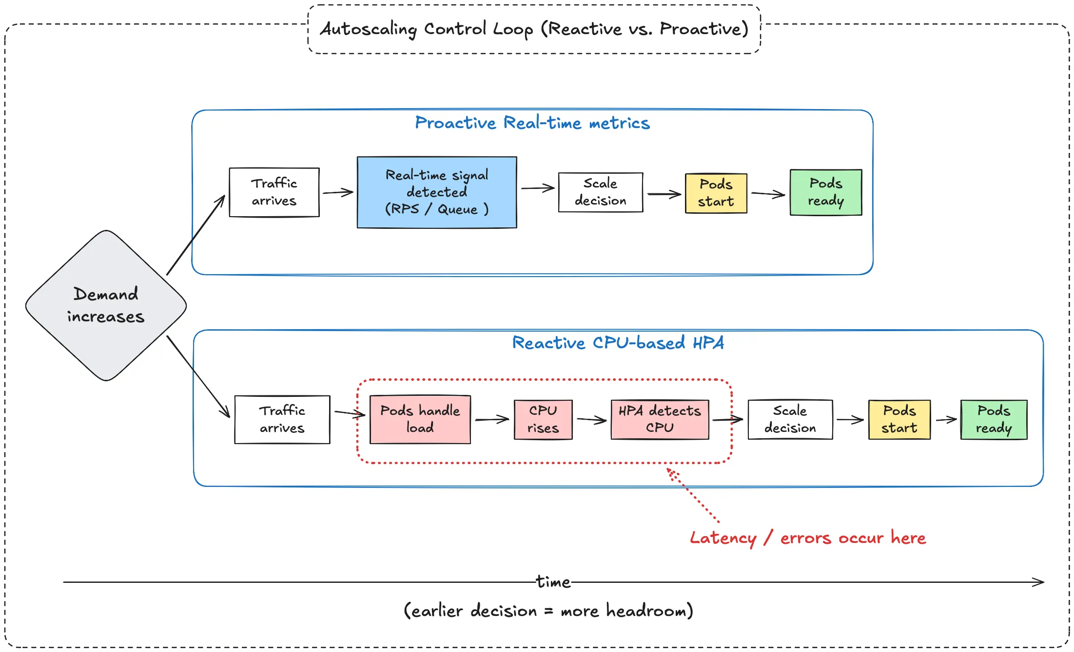
Why CPU / Memory HPA Is Often Late
CPU and memory are effects of work already happening. By the time they move, user demand has already arrived and existing pods are already absorbing the hit.
Sources of delay
- Lagging signal – CPU rises after demand arrives.
- Averaging effects – short spikes can be smoothed out.
- Pod readiness – capacity is unavailable until pods are fully ready.
What Proactive Metrics Change
Custom and real-time metrics shift scaling earlier by measuring incoming demand (or early pressure) directly, instead of waiting for downstream resource usage to rise.
Common examples:
- Request rate (RPS)
- Concurrent in-flight requests
- Queue depth or backlog
- Event lag
- Latency or SLO-related signals
- Predicted or forecasted demand
Why they reduce delay
- Earlier detection – demand is visible as soon as it arrives.
- Better burst sensitivity – spikes are less likely to be averaged away.
- Faster metric paths – often pushed/streamed, not scraped on long intervals.
- Pre-scaling capability – capacity can be added before saturation.
Reactive vs. Proactive (One Line)
CPU/memory HPA is a feedback loop (react after impact). Proactive signals act more like feed-forward control (scale when demand appears).
How Kedify Helps Reduce Autoscaling Delay
Kedify focuses on the part of the system that most strongly determines perceived “slowness”: the signal path (what you scale on, and how quickly it reaches the autoscaler).
Cut autoscaling delay where it starts.
Scale on workload signals (not just CPU) with Kedify.
Get StartedWhat Kedify changes
Kedify helps reduce delay by shifting scaling decisions earlier in the request or event lifecycle:
-
Low-latency workload signals: Deliver demand-oriented signals quickly, so the autoscaler can react before CPU saturation becomes visible.
-
Burst-aware behavior: Handle spikes without losing them to per-pod averaging and slow polling intervals.
-
Predictive / pre-scaling: Add headroom ahead of known patterns (deploy spikes, scheduled jobs, traffic waves).
-
Fits Kubernetes primitives: Works with Kubernetes autoscaling workflows while upgrading the quality and speed of the input signal.
Resulting Impact
Compared to native resource-based HPA, Kedify enables:
- Earlier scaling decisions
- Reduced latency and error spikes during bursts
- Better SLO adherence for user-facing and event-driven systems
Native HPA vs. Kedify
| Dimension | Native Kubernetes HPA (CPU/Memory) | Kedify |
|---|---|---|
| Signal | Resource utilization (CPU/memory) | Workload/demand signals (traffic, queues, lag) |
| Signal timing | Late (after impact) | Early (as demand appears) |
| Metric path | Periodic polling/scraping | Low-latency streamed/pushed |
| Bursts | Spikes can be averaged away | Burst-aware signals and scaling |
| User impact under spikes | Latency/errors before capacity rises | Capacity added earlier |
Example 1: User-Facing Microservices Application
Scenario
A user-facing web application consists of multiple microservices:
- API Gateway – receives HTTP requests
- Auth Service – validates users
- Processing Service – performs business logic
- Data Service – accesses storage
The system has an SLO that 95% of requests must complete within 300 ms. Traffic is usually steady but experiences sudden bursts.
- Demand rises → existing pods get busy first.
- CPU increases later and is averaged → HPA scales after the impact starts.
- New pods need startup + readiness → latency spikes before capacity arrives.
Outcome: Users see slower responses during the burst.
- Demand is visible immediately (RPS/concurrency) → autoscaler acts earlier.
- Replicas start before CPU saturation.
- Capacity lands closer to the start of the spike.
Outcome: Latency stays closer to the SLO during bursts.
Example 2: Queue- and Event-Driven System
Scenario
A background processing system consumes events from a message queue.
- Backlog grows first; workers get busy.
- CPU rises later → scaling starts after queue delay is already increasing.
- Workers start slowly relative to backlog growth.
Outcome: Queue lag grows and SLAs can be violated.
- Backlog/lag is visible immediately → scale on the thing users feel.
- Workers start earlier, while backlog is still manageable.
- Lag stays smaller during bursts.
Outcome: Queue delay stays closer to SLA.
If you want faster, smoother scaling, focus on when the autoscaler learns about demand. CPU/memory can only react after the system is already under pressure; demand-oriented signals let you scale closer to the start of the spike.
Talk to Us
Want to discuss your setup and how to reduce autoscaling delay in practice?
Don’t hesitate to book a demo with our team.